What is the time response (tau) of a thermistor?
The time constant of a thermistor, also referred to as time response or tau (τ), is conventionally defined as the amount of time for the signal measured by the thermistor to increase to 63.2% of its final value (Emery and Thomson, 2004). In other words, it is the e-folding time: 63.2% = 1 – 1/e.
Why does thermistor time response matter?
Tau essentially describes how quickly a thermistor responds to a change in temperature; thus, when selecting a thermistor, it might be important to consider what tau is necessary for the project and scientific goals. For example, if the sensors are being deployed in a rapidly changing environment or in a location with large changes in temperature over a small spatial scale, a fast thermistor time response time might be necessary to properly resolve all features. However, as fast-response thermistors are by necessity thinner and generally less durable than slower thermistors, if the region is more thermally stable or the sensors are deployed long-term in one location, a sensor with a slower response time might suffice.
How is thermistor time response determined?
Tau is calculated by analysing the exponential decay for a sensor immersed in a well-stirred constant temperature bath. From this experiment, it is possible to create a model of the response of a thermistor to changes in ambient temperature; this model can predict the response of a thermistor, similar to a single-pole low-pass filter. Examples of this methodology are given below for standard and fast RBR thermistors.
Standard thermistor
Standard RBR thermistors have a tau of less than 1s. Figure 1 shows the response of this type of thermistor when sampling at 16Hz and experiencing a step change of 20°C. The step change was induced by transferring the sensor from measuring in the air (at a temperature of 22°C) to a Hart Scientific 7012 calibration water bath maintained at 2°C.
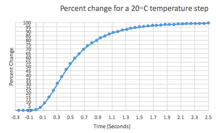
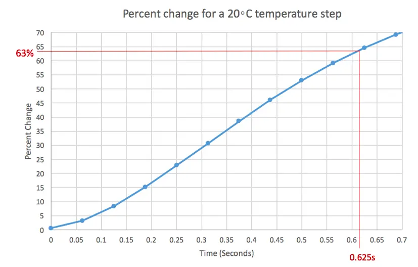
Figure 2 zooms in on the data presented in Figure 1 to highlight when the percent change is equal to 63%, indicating the time constant and highlighted in red. For this standard thermistor, the time constant is 625 milliseconds. The initial lag in thermistor response is due to the transfer to the bath being performed manually and not by an instantaneous step change.
The experiment was repeated with 15 RBRduet T.D temperature and depth loggers, all sampling at 16Hz. These experiments are summarised in Figure 3. The average e-folding time (i.e. time constant) amongst these experiments was 633 milliseconds with a standard deviation of 66 milliseconds.
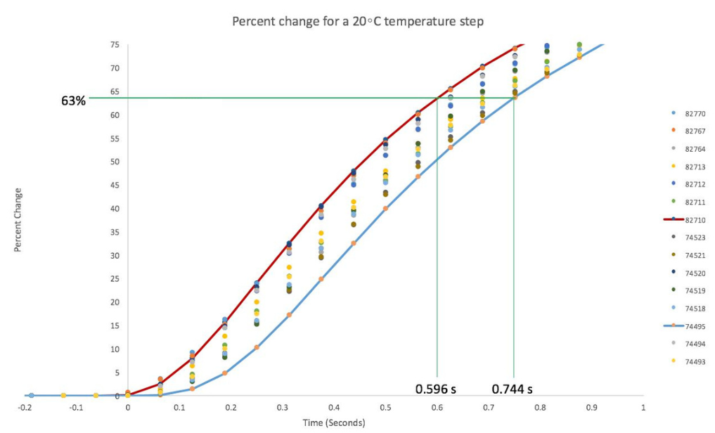
The calculated time constant, i.e. the e-folding time for a step change between two temperature regimes, is consistently lower than RBR’s nominal claim of 1s. It is important to note that the effective time constant of a thermistor depends on both the orientation of the sensor relative to the flow (e.g., parallel or perpendicular) and the speed of the flow past the thermistor. RBR’s experiments were designed to maximise the performance of the thermistor, which was achieved by minimising the influence of the sensor body and its guard, and by ensuring there was ample flow traversing the thermistor.
Fast thermistor
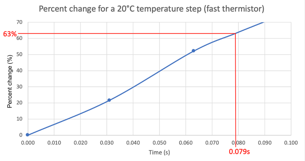
RBR’s calibration team performed the same experiment on the fast thermistor, and found that the response time of RBR’s fast thermistor is less than 0.1s when sampling at 16Hz and experiencing a step change of 20°C induced by transferring the sensor from measuring in the air (at a temperature of 22°C) to a Hart Scientific 7012 calibration water bath maintained at 2°C (Figure 4).
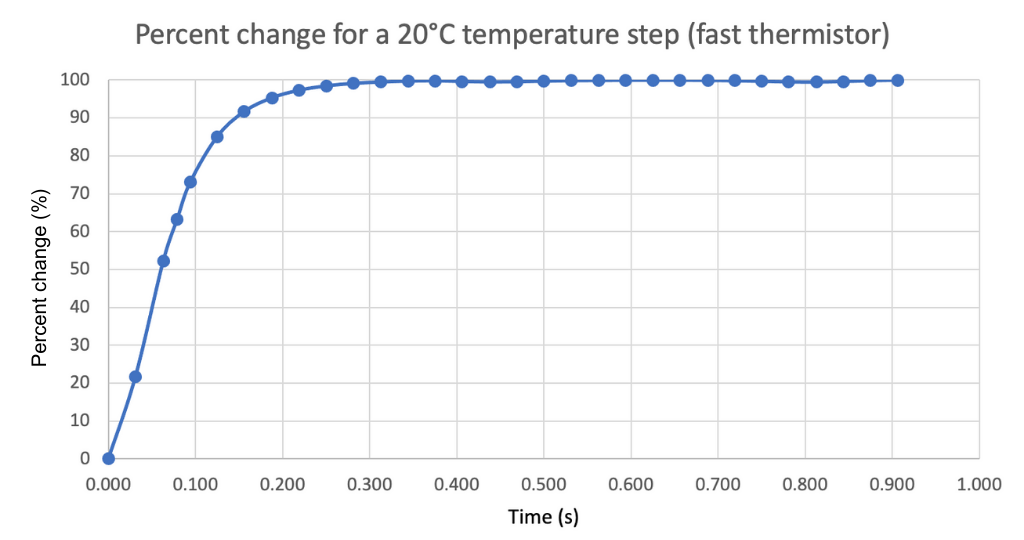
Figure 5 again zooms in on the data from Figure 4 to highlight the e-folding time of 63% (i.e. the time constant), as indicated by the red line. For the fast thermistor, the time constant is 79 milliseconds. Note there is a similar initial lag at the beginning of the time series due to the non-idealized conditions.
From repeated experiments, the team found that the e-folding time for the step change between the two temperature regimes is consistently lower than RBR’s nominal claim of 0.1 seconds.
What is the spectral response of a thermistor?
The spectral response of a thermistor is the ability of the sensor to accurately resolve temperature fluctuations at different frequencies. Due to the exponential response of thermistors, the spectral response of these sensors varies as a function of frequency. We thus define the bandwidth as the frequency at which the spectral response of a thermistor is half the input signal – also referred to as the “3dB frequency”. For the single-pole exponential response typically used for a thermistor, the value of the 3dB frequency is 1/(2πτ), where τ is the time constant.
Assessing the spectral response, particularly the bandwidth, of a sensor requires comparison against a reference source for which the response is well characterised. Any deviations from the ideal single-pole model will result in apparent discrepancies from the theoretical 3 dB frequency. For example, Lueck et al. (1977) note that the frequency response of a single pole filter representation is in error by about 10% at 1.25 times the 3dB frequency, and the error increases with increasing frequency.
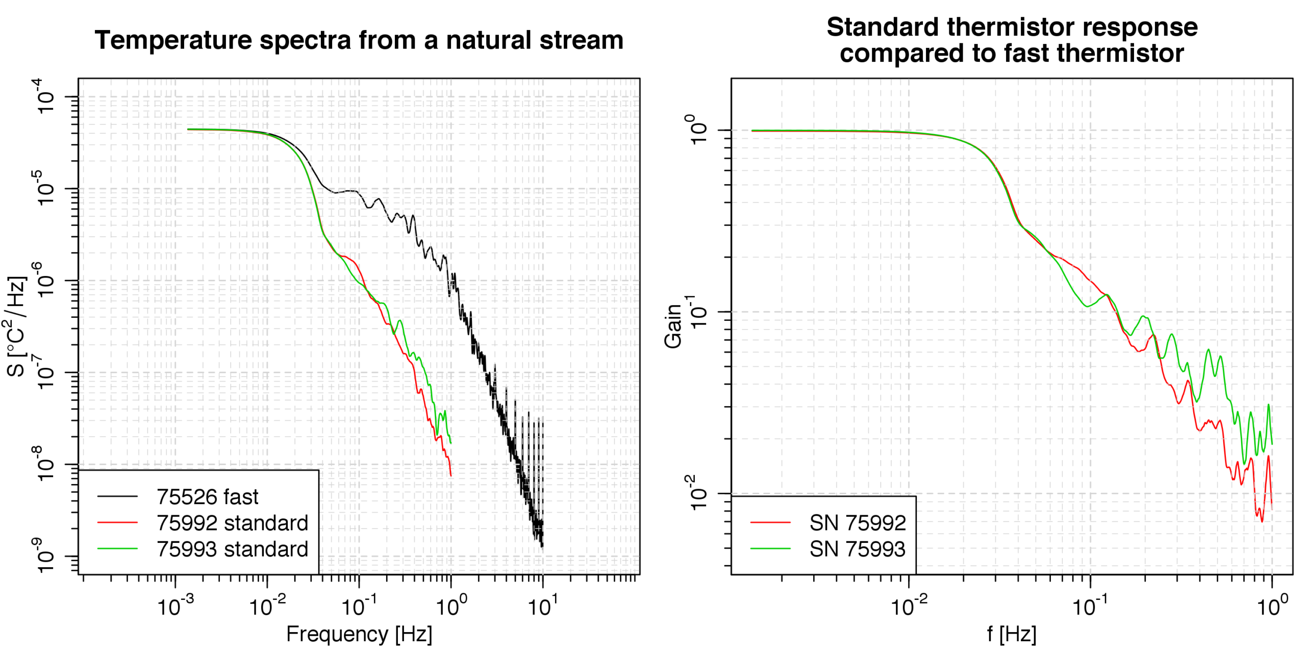
To illustrate the different frequency responses of the two RBR thermistors (standard vs. fast), loggers were deployed in tandem in a natural stream. The spectra for each sensor (one fast thermistor and two standard thermistors) are shown in Figure 6a. Figure 6b shows the spectra from the standard thermistors divided by the spectrum from the fast thermistor (i.e. the gain ratio), which estimates the gain of the thermistor response. At a frequency of 1Hz, which is the Nyquist frequency for a 2Hz sampling instrument, the spectral response of a standard thermistor is ~ 100 times lower than the fast thermistor. These are important considerations when planning deployments where high frequency variability might be of interest.
References and additional materials
Emery, William J., and Richard E. Thomson. (2004). Data Analysis Methods in Physical Oceanography. Amsterdam, NL: Elsevier.
Lueck, Rolf G., Owen Hertzman, and Thomas R. Osborn. The spectral response of thermistors. Deep Sea Research 24.10 (1977): 951-970.
Steinhart, John S., Stanley R. Hart. Calibration curves for thermistors. Deep-Sea Research and Oceanographic Abstracts 15.4 (1968): 497–503. https://doi.org/10.1016%2F0011-7471%2868%2990057-0